فئة ماندلبرو

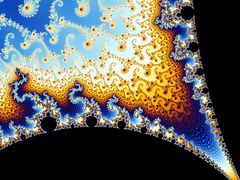
مجموعة ماندلبرو Mandelbrot set إحدى الأسكال الكسيرية المشهورة بشكل واسع حتى خارج مجال علماء الرياضيات لتداخلها مع ما يدعى الفن الكسيري حيث تعمد لتقديم صور فنية تتميز بالجمال و التجريدية . ما يميز مجموعة ماندلبرو هو البنية المعقدة التي تقدمها رغم بساطة تعريفها .

Initial image of a Mandelbrot set zoom sequence with a continuously colored environment

Progressive infinite iterations of the "Nautilus" section of the Mandelbrot Set rendered using webGL

Mandelbrot animation based on a static number of iterations per pixel

تفصيلة فئة ماندلبرو

لمجموعة ماندلبرو مكانتها حاليا في دراسة الديناميك العقدي complex dynamics الحقل الذي اهتم به الرياضياتي الفرنسي پيير فاتو Pierre Fatou و گاستون جوليا Gaston Julia في بداية القرن العشرين . أول صور مجموعة ماندلبرو قام برسمها كل من بروكس و ماتلسكي كجزء من دراستهم لزمرة كلاينيان Kleinian group

قام ماندلبرو لاحقا بدراسة فضاء المتغيرات لعديات الحدود التربيعية في مقالة ظهرت عام 1980 لكن الدراسة الرياضية الحقيقية لمجموعة ماندلبرو بدأت مع عمل كل من أدريان دوادي Adrien Douady و جون ه. هبرد John H. Hubbard اللذان قاما بتأسيس وإيضاح العديد من خواص $M$ ، وأسمياها مجموعة ماندلبرو.

More precisely, the Mandelbrot set is the set of values of c in the complex plane for which the orbit of 0 under iteration of the quadratic map

$z_{n+1}=z_{n}^{2}+c$

remains bounded. That is, a complex number c is part of the Mandelbrot set if, when starting with z₀ = 0 and applying the iteration repeatedly, the absolute value of z_n remains bounded however large n gets. This can also be represented as

$z_{n+1}=z_{n}^{2}+c,$

$c\in M\iff \lim _{n\to \infty }|z_{n+1}|\leq 2.$

For example, letting c = 1 gives the sequence 0, 1, 2, 5, 26,…, which tends to infinity. As this sequence is unbounded, 1 is not an element of the Mandelbrot set. On the other hand, c = −1 gives the sequence 0, −1, 0, −1, 0,…, which is bounded, and so −1 belongs to the Mandelbrot set.

. . . . . . . . . . . . . . . . . . . . . . . . . . . . . . . . . . . . . . . . . . . . . . . . . . . . . . . . . . . . . . . . . . . . . . . . . . . . . . . . . . . . . . . . . . . . . . . . . . . . . . . . . . . . . . . . . . . . . . . . . . . . . . . . . . . . . . . . . . . . . . . . . . . . . . . . . . . . . . . . . . . . . . . .

 تاريخ

The first published picture of the Mandelbrot set, by Robert W. Brooks and Peter Matelski in 1978

لمجموعة ماندلبرو مكانها في الديناميكا العقدية, وهو مجال بُحث فيه لأول مرة من طرف عالمي الرياضيات الفرنسيين پيير فاتو وگاستون جوليا في بداية القرن العشرين. أول صورة لهاته الكسيرية رُسمت من طرف روبرت وولف بروكس وپيتر ماتلسكي، وكان ذلك في عام 1978, كجزء من دراسة للزمر الكلاينية. في أول يوم من مارس عام 1980، رأى ماندلبرو رسما للمجموعة لأول مرة, وكان ذلك في مختبر تابع لـ آي‌ بي‌ إم في نيويورك بالولايات المتحدة.

درس ماندلبرو فضاء البارمترات لمتعددات الحدود التربيعية في مقالة ظهرت عام 1980.

لكن الدراسة الرياضية الحقيقية لمجموعة ماندلبرو بدأت مع عمل كل من أدريان دوادي وجون ه. هوبارد John H. Hubbard اللذان قاما بتأسيس وإيضاح العديد من خواص $M$، وأسمياها مجموعة ماندلبرو تكريما لماندلبرو.

 التعريف الشكلي

The Mandelbrot set $M$ is defined by a family of complex quadratic polynomials

$P_{c}:\mathbb {C} \to \mathbb {C}$

المعطى من

$P_{c}:z\mapsto z^{2}+c,$

where $c$ is a complex parameter. For each $c$, one considers the behavior of the sequence

$(0,P_{c}(0),P_{c}(P_{c}(0)),P_{c}(P_{c}(P_{c}(0))),\ldots )$

A mathematician's depiction of the Mandelbrot set M. A point c is colored black if it belongs to the set, and white if not. Re[c] and Im[c] denote the real and imaginary parts of c, respectively.

 الخصائص الأساسية

The Mandelbrot set is a compact set, since it is closed and contained in the closed disk of radius 2 around the origin. More specifically, a point $c$ belongs to the Mandelbrot set if and only if

$|P_{c}^{n}(0)|\leq 2$ for all $n\geq 0.$

In other words, if the absolute value of $P_{c}^{n}(0)$ ever becomes larger than 2, the sequence will escape to infinity.

Correspondence between the Mandelbrot set and the bifurcation diagram of the logistic map

The intersection of $M$ with the real axis is precisely the interval [−2, 1/4]. The parameters along this interval can be put in one-to-one correspondence with those of the real logistic family,

$z\mapsto \lambda z(1-z),\quad \lambda \in [1,4].$

The correspondence is given by

$c={\frac {\lambda }{2}}\left(1-{\frac {\lambda }{2}}\right).$

In fact, this gives a correspondence between the entire parameter space of the logistic family and that of the Mandelbrot set.

As of October 2012, the area of the Mandelbrot is estimated to be 1.5065918849 ± 0.0000000028.

 خصائص أخرى

 Main cardioid and period bulbs

Periods of hyperbolic components

Upon looking at a picture of the Mandelbrot set, one immediately notices the large cardioid-shaped region in the center. This main cardioid is the region of parameters $c$ for which $P_{c}$ has an attracting fixed point. It consists of all parameters of the form

$c={\frac {\mu }{2}}\left(1-{\frac {\mu }{2}}\right)$

for some $\mu$ in the open unit disk.

There are infinitely many other bulbs tangent to the main cardioid: for every rational number ${\tfrac {p}{q}}$, with p and q coprime, there is such a bulb that is tangent at the parameter

$c_{\frac {p}{q}}={\frac {e^{2\pi i{\frac {p}{q}}}}{2}}\left(1-{\frac {e^{2\pi i{\frac {p}{q}}}}{2}}\right).$

Attracting cycle in 2/5-bulb plotted over Julia set (animation)

This bulb is called the ${\tfrac {p}{q}}$-bulb of the Mandelbrot set. It consists of parameters that have an attracting cycle of period $q$ and combinatorial rotation number ${\tfrac {p}{q}}$. More precisely, the $q$ periodic Fatou components containing the attracting cycle all touch at a common point (commonly called the $\alpha$-fixed point). If we label these components $U_{0},\dots ,U_{q-1}$ in counterclockwise orientation, then $P_{c}$ maps the component $U_{j}$ to the component $U_{j+p\,(\operatorname {mod} q)}$.

Attracting cycles and Julia sets for parameters in the 1/2, 3/7, 2/5, 1/3, 1/4, and 1/5 bulbs

Cycle periods and antennae

The change of behavior occurring at $c_{\frac {p}{q}}$ is known as a bifurcation: the attracting fixed point "collides" with a repelling period q-cycle. As we pass through the bifurcation parameter into the ${\tfrac {p}{q}}$-bulb, the attracting fixed point turns into a repelling fixed point (the $\alpha$-fixed point), and the period q-cycle becomes attracting.

 الترابط المحلي

نموذج طبولوجي لفئة ماندلبرو بدون فئات ماندلبرو صغرى ونقاط Misiurewicz (نموذج شجرة الصبار)

نموذج ثرستون لفئة ماندلبرو (فئة ماندلبرو مجرّد)

 التشابه الذاتي

Self similarity in the Mandelbrot set shown by zooming in on a round feature while panning in the negative-x direction. The display center pans from (−1, 0) to (−1.31, 0) while the view magnifies from 0.5 × 0.5 to 0.12 × 0.12 to approximate the Feigenbaum ratio $\delta$.

Self-similarity around Misiurewicz point −0.1011 + 0.9563i.

 المزيد من النتائج

A zoom into the Mandelbrot set illustrating a Julia "island" and the corresponding Julia set of the form $f_{c}(z)=z^{2}+c\,$, in which c is the centre of the Mandelbrot set zoom-in

. . . . . . . . . . . . . . . . . . . . . . . . . . . . . . . . . . . . . . . . . . . . . . . . . . . . . . . . . . . . . . . . . . . . . . . . . . . . . . . . . . . . . . . . . . . . . . . . . . . . . . . . . . . . . . . . . . . . . . . . . . . . . . . . . . . . . . . . . . . . . . . . . . . . . . . . . . . . . . . . . . . . . . . .

 الهندسة

Components on main cardioid for periods 8–14 with antennae 7–13

 معرض صور لتتابع مكبَّر

The Mandelbrot set shows more intricate detail the closer one looks or magnifies the image, usually called "zooming in". The following example of an image sequence zooming to a selected c value gives an impression of the infinite richness of different geometrical structures and explains some of their typical rules.

The magnification of the last image relative to the first one is about 10¹⁰ to 1. Relating to an ordinary monitor, it represents a section of a Mandelbrot set with a diameter of 4 million kilometres. Its border would show an astronomical number of different fractal structures.

• 

  Start. Mandelbrot set with continuously colored environment.

• 

  Gap between the "head" and the "body", also called the "seahorse valley"

• 

  Double-spirals on the left, "seahorses" on the right

• 

  "Seahorse" upside down

The seahorse "body" is composed by 25 "spokes" consisting of two groups of 12 "spokes" each and one "spoke" connecting to the main cardioid. These two groups can be attributed by some kind of metamorphosis to the two "fingers" of the "upper hand" of the Mandelbrot set; therefore, the number of "spokes" increases from one "seahorse" to the next by 2; the "hub" is a so-called Misiurewicz point. Between the "upper part of the body" and the "tail" a distorted small copy of the Mandelbrot set called satellite may be recognized.

• 

  The central endpoint of the "seahorse tail" is also a Misiurewicz point.

• 

  Part of the "tail" — there is only one path consisting of the thin structures that lead through the whole "tail". This zigzag path passes the "hubs" of the large objects with 25 "spokes" at the inner and outer border of the "tail"; thus the Mandelbrot set is a simply connected set, which means there are no islands and no loop roads around a hole.

• 

  Satellite. The two "seahorse tails" are the beginning of a series of concentric crowns with the satellite in the center. Open this location in an interactive viewer.

• 

  Each of these crowns consists of similar "seahorse tails"; their number increases with powers of 2, a typical phenomenon in the environment of satellites. The unique path to the spiral center passes the satellite from the groove of the cardioid to the top of the "antenna" on the "head".

• 

  "Antenna" of the satellite. Several satellites of second order may be recognized.

• 

  The "seahorse valley" of the satellite. All the structures from the start of the zoom reappear.

• 

  Double-spirals and "seahorses" – unlike the 2nd image from the start, they have appendices consisting of structures like "seahorse tails"; this demonstrates the typical linking of n + 1 different structures in the environment of satellites of the order n, here for the simplest case n = 1.

• 

  Double-spirals with satellites of second order – analogously to the "seahorses", the double-spirals may be interpreted as a metamorphosis of the "antenna"

• 

  In the outer part of the appendices, islands of structures may be recognized; they have a shape like Julia sets J_c; the largest of them may be found in the center of the "double-hook" on the right side

• 

  Part of the "double-hook"

• 

  Islands; see below

 تعميمات

Animation of the Mandelbrot set for d from 0 to 5

Animation of the set for d from 0.05 to 2

Multibrot sets are bounded sets found in the complex plane for members of the general monic univariate polynomial family of recursions

$z\mapsto z^{d}+c.\$

 Other, non-analytic, mappings

Of particular interest is the tricorn fractal, the connectedness locus of the anti-holomorphic family

$z\mapsto {\bar {z}}^{2}+c.$

The tricorn (also sometimes called the Mandelbar set) was encountered by Milnor in his study of parameter slices of real cubic polynomials. It is not locally connected. This property is inherited by the connectedness locus of real cubic polynomials.

Another non-analytic generalization is the Burning Ship fractal, which is obtained by iterating the mapping

$z\mapsto (|\Re \left(z\right)|+i|\Im \left(z\right)|)^{2}+c.$

The Multibrot set is obtained by varying the value of the exponent d. The article has a video that shows the development from d = 0 to 7 at which point there are 6 i.e. (d − 1) lobes around the perimeter. A similar development with negative exponents results in (1 − d) clefts on the inside of a ring.

 رسوم حاسوبية

Still image of a movie of increasing magnification on 0.001643721971153 − 0.822467633298876i

Still image of an animation of increasing magnification

In pseudocode, this algorithm would look as follows. The algorithm does not use complex numbers and manually simulates complex-number operations using two real numbers, for those who do not have a complex data type. The program may be simplified if the programming language includes complex-data-type operations.

For each pixel (Px, Py) on the screen, do:
{
  x0 = scaled x coordinate of pixel (scaled to lie in the Mandelbrot X scale (-2.5, 1))
  y0 = scaled y coordinate of pixel (scaled to lie in the Mandelbrot Y scale (-1, 1))
  x = 0.0
  y = 0.0
  iteration = 0
  max_iteration = 1000
  while (x*x + y*y < 2*2  AND  iteration < max_iteration) {
    xtemp = x*x - y*y + x0
    y = 2*x*y + y0
    x = xtemp
    iteration = iteration + 1
  }
  color = palette[iteration]
  plot(Px, Py, color)
}

Here, relating the pseudocode to $c$, $z$ and $P_{c}$:

• $z=x+iy\$
• $z^{2}=x^{2}+i2xy-y^{2}\$
• $c=x_{0}+iy_{0}\$

and so, as can be seen in the pseudocode in the computation of x and y:

• $x=\mathop {\mathrm {Re} } (z^{2}+c)=x^{2}-y^{2}+x_{0}$ and $y=\mathop {\mathrm {Im} } (z^{2}+c)=2xy+y_{0}.\$

To get colorful images of the set, the assignment of a color to each value of the number of executed iterations can be made using one of a variety of functions (linear, exponential, etc.). One practical way, without slowing down calculations, is to use the number of executed iterations as an entry to a look-up color palette table initialized at startup. If the color table has, for instance, 500 entries, then the color selection is n mod 500, where n is the number of iterations.

 تلوين متصل (ناعم)

This image was rendered with the escape time algorithm. Notice the very obvious "bands" of color

This image was rendered with the normalized iteration count algorithm. Notice the bands of color have been replaced by a smooth gradient. Also, the colors take on the same pattern that would be observed if the escape time algorithm were used.

$\phi (z)=\lim _{n\to \infty }(\log |z_{n}|/P^{n}),$

where z_n is the value after n iterations and P is the power for which z is raised to in the Mandelbrot set equation (z_n+1 = zn^P + c, P is generally 2).

If we choose a large bailout radius N (e.g., 10¹⁰⁰), we have that

$\log |z_{n}|/P^{n}=\log(N)/P^{\nu (z)}$

for some real number $\nu (z)$, and this is

$\nu (z)=n-\log _{P}(\log |z_{n}|/\log(N)),$

and as n is the first iteration number such that |z_n| > N, the number we subtract from n is in the interval [0, 1).

For example, modifying the above pseudocode and also using the concept of linear interpolation would yield

For each pixel (Px, Py) on the screen, do:
{
  x0 = scaled x coordinate of pixel (scaled to lie in the Mandelbrot X scale (-2.5, 1))
  y0 = scaled y coordinate of pixel (scaled to lie in the Mandelbrot Y scale (-1, 1))
  x = 0.0
  y = 0.0
  iteration = 0
  max_iteration = 1000
  // Here N=2^8 is chosen as a reasonable bailout radius.
  while ( x*x + y*y < (1 << 16)  AND  iteration < max_iteration ) {
    xtemp = x*x - y*y + x0
    y = 2*x*y + y0
    x = xtemp
    iteration = iteration + 1
  }
  // Used to avoid floating point issues with points inside the set.
  if ( iteration < max_iteration ) {
    // sqrt of inner term removed using log simplification rules.
    log_zn = log( x*x + y*y ) / 2
    nu = log( log_zn / log(2) ) / log(2)
    // Rearranging the potential function.
    // Dividing log_zn by log(2) instead of log(N = 1<<8)
    // because we want the entire palette to range from the
    // center to radius 2, NOT our bailout radius.
    iteration = iteration + 1 - nu
  }
  color1 = palette[floor(iteration)]
  color2 = palette[floor(iteration) + 1]
  // iteration % 1 = fractional part of iteration.
  color = linear_interpolate(color1, color2, iteration % 1)
  plot(Px, Py, color)
}

. . . . . . . . . . . . . . . . . . . . . . . . . . . . . . . . . . . . . . . . . . . . . . . . . . . . . . . . . . . . . . . . . . . . . . . . . . . . . . . . . . . . . . . . . . . . . . . . . . . . . . . . . . . . . . . . . . . . . . . . . . . . . . . . . . . . . . . . . . . . . . . . . . . . . . . . . . . . . . . . . . . . . . . .

 تقدير المسافة الداخلية

Pixels colored according to the estimated interior distance

It is also possible to estimate the distance of a limitly periodic (i.e., inner) point to the boundary of the Mandelbrot set. The estimate is given by

$b={\frac {1-\left|{{\frac {\partial }{\partial {z}}}P_{c}^{p}(z_{0})}\right|^{2}}{\left|{{\frac {\partial }{\partial {c}}}{\frac {\partial }{\partial {z}}}P_{c}^{p}(z_{0})+{\frac {\partial }{\partial {z}}}{\frac {\partial }{\partial {z}}}P_{c}^{p}(z_{0}){\frac {{\frac {\partial }{\partial {c}}}P_{c}^{p}(z_{0})}{1-{\frac {\partial }{\partial {z}}}P_{c}^{p}(z_{0})}}}\right|}},$

where

• $p$ is the period,
• $c$ is the point to be estimated,
• $P_{c}(z)$ is the complex quadratic polynomial $P_{c}(z)=z^{2}+c$
• $P_{c}^{p}(z_{0})$ is the $p$-fold iteration of $P_{c}(z)\to z$, starting with $P_{c}^{0}(z)=z_{0}$
• $z_{0}$ is any of the $p$ points that make the attractor of the iterations of $P_{c}(z)\to z$ starting with $P_{c}^{0}(z)=c$; $z_{0}$ satisfies $z_{0}=P_{c}^{p}(z_{0})$,
• ${\frac {\partial }{\partial {c}}}{\frac {\partial }{\partial {z}}}P_{c}^{p}(z_{0})$, ${\frac {\partial }{\partial {z}}}{\frac {\partial }{\partial {z}}}P_{c}^{p}(z_{0})$, ${\frac {\partial }{\partial {c}}}P_{c}^{p}(z_{0})$ and ${\frac {\partial }{\partial {z}}}P_{c}^{p}(z_{0})$ are various derivatives of $P_{c}^{p}(z)$, evaluated at $z_{0}$.

3D view: smallest absolute value of the orbit of the interior points of the Mandelbrot set

 تقفي الحدود / التأكد من الحواف

Edge detection using Sobel filter of hyperbolic components of Mandelbrot set

 انظر أيضاً

• Collatz fractal
• Gilbreath permutation, a combinatorial object that can be used to count the real periodic points of the Mandelbrot set
• Mandelbox
• Mandelbulb
• Newton fractal
• Orbit portrait
• Orbit trap
• Pickover stalk

 للاستزادة

• John W. Milnor, Dynamics in One Complex Variable (Third Edition), Annals of Mathematics Studies 160, (Princeton University Press, 2006), ISBN 0-691-12488-4
  (First appeared in 1990 as a Stony Brook IMS Preprint, available as arXiV:math.DS/9201272 )
• Nigel Lesmoir-Gordon, The Colours of Infinity: The Beauty, The Power and the Sense of Fractals, ISBN 1-904555-05-5
  (includes a DVD featuring Arthur C. Clarke and David Gilmour)
• Heinz-Otto Peitgen, Hartmut Jürgens, Dietmar Saupe, Chaos and Fractals - New Frontiers of Science (Springer, New-York, 1992, 2004), ISBN 0-387-20229-3

 وصلات خارجية

• Chaos and Fractals at the Open Directory Project
• The Mandelbrot Set and Julia Sets by Michael Frame, Benoit Mandelbrot, and Nial Neger
• Video: Mandelbrot fractal zoom to 6.066 e228
• मण्डलबेथ (maṇḍalabeth) 3D analog of the mandelbrot set, with various symmetry groups