تحويل لاپلاس
في الرياضيات، تحويل لاپلاس Laplace transform عملية تجرى على الدوال الرياضية لتحويلها من مجال إلى آخر، وعادة يكون التحويل من مجال الزمن إلى مجال التردد، وهو شبيه بتحويل فوريي إلا أنه تم تطويرهما بشكل مستقل. وتحويل لابلاس مفيد في تحليل النظم الخطية (بخلاف تحويل فوريي الذي يستخدم عادة في تحليل الإشارات)، كما يستخدم لحل المعادلات التفاضلية لأنه يحولها إلى معادلات جبرية. وسمي التحويل بهذا الاسم نسبة إلى العالم الفرنسي لابلاس الذي عاش في القرن التاسع عشر. The transform has many applications in science and engineering because it is a tool for solving differential equations.[1] In particular, it transforms ordinary differential equations into algebraic equations and convolution into multiplication.[2][3] For suitable functions f, the Laplace transform is the integral

. . . . . . . . . . . . . . . . . . . . . . . . . . . . . . . . . . . . . . . . . . . . . . . . . . . . . . . . . . . . . . . . . . . . . . . . . . . . . . . . . . . . . . . . . . . . . . . . . . . . . . . . . . . . . . . . . . . . . . . . . . . . . . . . . . . . . . . . . . . . . . . . . . . . . . . . . . . . . . . . . . . . . . . .
التاريخ

The Laplace transform is named after mathematician and astronomer پيير-سيمون، ماركي دى لاپلاس، who used a similar transform in his work on probability theory.[4] Laplace wrote extensively about the use of generating functions in Essai philosophique sur les probabilités (1814), and the integral form of the Laplace transform evolved naturally as a result.[5]
Laplace's use of generating functions was similar to what is now known as the z-transform, and he gave little attention to the continuous variable case which was discussed by Niels Henrik Abel.[6] The theory was further developed in the 19th and early 20th centuries by Mathias Lerch,[7] Oliver Heaviside,[8] and Thomas Bromwich.[9]
The current widespread use of the transform (mainly in engineering) came about during and soon after World War II,[10] replacing the earlier Heaviside operational calculus. The advantages of the Laplace transform had been emphasized by Gustav Doetsch,[11] to whom the name Laplace transform is apparently due.
From 1744, Leonhard Euler investigated integrals of the form


These types of integrals seem first to have attracted Laplace's attention in 1782, where he was following in the spirit of Euler in using the integrals themselves as solutions of equations.[15] However, in 1785, Laplace took the critical step forward when, rather than simply looking for a solution in the form of an integral, he started to apply the transforms in the sense that was later to become popular. He used an integral of the form

Laplace also recognised that Joseph Fourier's method of Fourier series for solving the diffusion equation could only apply to a limited region of space, because those solutions were periodic. In 1809, Laplace applied his transform to find solutions that diffused indefinitely in space.[17]
التعريف الشكلي
The Laplace transform of a function f(t), defined for all real numbers t ≥ 0, is the function F(s), which is a unilateral transform defined by
|
|
(Eq.1) |

where s is a complex number frequency parameter

An alternate notation for the Laplace transform is instead of F.[3]

The meaning of the integral depends on types of functions of interest. A necessary condition for existence of the integral is that f must be locally integrable on قالب:Closed-open. For locally integrable functions that decay at infinity or are of exponential type ( ), the integral can be understood to be a (proper) Lebesgue integral. However, for many applications it is necessary to regard it as a conditionally convergent improper integral at ∞. Still more generally, the integral can be understood in a weak sense, and this is dealt with below.

One can define the Laplace transform of a finite Borel measure μ by the Lebesgue integral[18]

An important special case is where μ is a probability measure, for example, the Dirac delta function. In operational calculus, the Laplace transform of a measure is often treated as though the measure came from a probability density function f. In that case, to avoid potential confusion, one often writes


This limit emphasizes that any point mass located at 0 is entirely captured by the Laplace transform. Although with the Lebesgue integral, it is not necessary to take such a limit, it does appear more naturally in connection with the Laplace–Stieltjes transform.
مقدمة
إذا اعتبرنا أن t الزمن
، وأن s عددا مركبا
فإن تحويل لاپلاس الذي نرمز له هنا بالرمز L هو عملية تحويل إشارة أو دالة من دالة بمتغير هو الزمن إلى دالة بمتغير آخر هو التردد، أما الأصح هو أنها مؤثر يحول دالة بمتغير قيمته عدد حقيقي إلى دالة بمتغير قيمته (عدد مركب).
تحويل الدالة من متغير في الزمن إلى دالة في متغير للمسافة مثلا
مثال ذلك
تحويل السرعة المتغيرة التي هي دالة في الزمن
إلى دالة في المسافة
تحويل درجة الحرارة من دالة في الزمن إلى دالة في درجة حرارة المصدر
و دالة التحويل L أي التي تحول دالة بمتغير هو الزمن إلى دالة بمتغير هو التردد يمكن حسابها على النحو الآتي:
و كما يوجد تحويل لابلاس فإنه يوجد تحويل لابلاس معاكس، ويُرمز له بالرمز وهو يقوم بالتحويل العكسي لتحويل لابلاس أي من دالة بمتغير قيمته عدد مركب إلى دالة بمتغير قيمته عدد حقيقي، ويمكن حساب هذه العملية على النحو التالي:


خصائص ونظريات
هناك مجموعة من الخصائص لتحويل لابلاس لابد من معرفتها لتسهيل استخدامه وبخاصة في تحليل النظم الخطية، من أهمها حالات التفاضل والتكامل.
والجدول التالي يبين ملخصا لهذه الخصائص والنظريات:
إذا كان هناك دالتين:
(f(t و (g(t وكان تحويل لابلاس لهما هو: (F(s و (G(s


وفيما يلي بيان تلك الخصائص والنظريات transform:[19]
| مجال الزمن t | مجال التردد s | ملاحظات | |
|---|---|---|---|
| الخطية | يمكن إثباتها بالقواعد الأساسية للتكامل. | ||
| التفاضل (الاشتقاق) في مجال التردد | F′ هي المشتقة الأولى لـ F. | ||
| التفاضل (الاشتقاق) في مجال التردد | F(n)′ هي المشتقة رقم n لـ F. | ||
| التفاضل (الاشتقاق) في مجال الزمن | بفرض f قابلة للاشتقاق، ومشتقاتها على صورة دالة أسية للثابت الطبيعي e. ويمكن إثبات ذلك بواسطة التكامل بالتجزيء | ||
| التفاضل (الاشتقاق) الثاني في مجال الزمن | بفرض f قابلة للاشتقاق مرتين، ومشتقاتها الثانية على صورة دالة أسية للثابت الطبيعي e | ||
| التفاضل (الاشتقاق) عامةً في مجال الزمن | بفرض f قابلة للاشتقاق n من المرات، ومشتقاتها رقم n على صورة دالة أسية. | ||
| تكامل في مجال التردد | يمكن استنتاجه باستخدام التفاضل في مجال التردد. | ||
| التكامل في مجال الزمن | u(t) هي دالة قفزة. لاحظ أن: (u ∗ f)(t) يمثل التفاف (رياضيات) of u(t) و f(t). | ||
| تحجيم الزمن | |||
| إزاحة التردد | |||
| إزاحة الزمن | u(t) هي دالة قفزة أحادية | ||
| ضرب | التكامل يتم على الخط الرأسي Re(σ) = c الذي يقع في منطقة تقارب F.[20] | ||
| التفاف (رياضيات) | |||
| مرافق عدد مركب | |||
| ارتباط (إحصاء) | |||
| دالة دورية | f(t) هي دالة دورية زمنها الدوري هو T أي أن f(t) = f(t + T), لكل t ≥ 0. |


بعض الدوال ومقابلها في تحويل لابلاس


أهمية وفوائد تحويل لابلاس
تسهيل حل المعادلات التفاضلية
فلنعتبر مثلا المعادلة التفاضلية التالية:

مع اعتبار الحالة أو قيمة x في الزمن 0 أي أخذ ما يسمى بال initial conditions بعين الاعتبار:
و


إعطاء الحل مباشرة لهذه المعادلة (التي قد تكون مثلا معادلة جسم يقوم بحركة ما أي أنها نموذج عنه) قد يكون صعبا فما العمل? الحل هو تحويل المعادلة عن طريق تحويل لابلاس فتصير المعادلة كالاتي:

و ذلك عملا بالقاعدة التي تقول
وبذلك كل ما تبقى فعله الآن هو حل معادلة غير تفاضلية بسيطة وهي معادلة بولينوم من الدرجة الثانية.
طرق رياضياتية مساعدة
كثيرا ما نحتاج إلى استخدام طريقة إكمال المربع عند حساب تحويلات لابلاس العسكية، وذلك لوضع الدالة المراد تحويلها في صورة مربعة تناسب أحد الصور الموجودة بالجدول السابق.
العلاقة بالتحويلات الأخرى
. . . . . . . . . . . . . . . . . . . . . . . . . . . . . . . . . . . . . . . . . . . . . . . . . . . . . . . . . . . . . . . . . . . . . . . . . . . . . . . . . . . . . . . . . . . . . . . . . . . . . . . . . . . . . . . . . . . . . . . . . . . . . . . . . . . . . . . . . . . . . . . . . . . . . . . . . . . . . . . . . . . . . . . .
تحويل لاپلاس-ستيلتشس
The (unilateral) Laplace–Stieltjes transform of a function g : ℝ → ℝ is defined by the Lebesgue–Stieltjes integral

The function g is assumed to be of bounded variation. If g is the antiderivative of f:

then the Laplace–Stieltjes transform of g and the Laplace transform of f coincide. In general, the Laplace–Stieltjes transform is the Laplace transform of the Stieltjes measure associated to g. So in practice, the only distinction between the two transforms is that the Laplace transform is thought of as operating on the density function of the measure, whereas the Laplace–Stieltjes transform is thought of as operating on its cumulative distribution function.[21]
تحويل فورييه
The Fourier transform is a special case (under certain conditions) of the bilateral Laplace transform. While the Fourier transform of a function is a complex function of a real variable (frequency), the Laplace transform of a function is a complex function of a complex variable. The Laplace transform is usually restricted to transformation of functions of t with t ≥ 0. A consequence of this restriction is that the Laplace transform of a function is a holomorphic function of the variable s. Unlike the Fourier transform, the Laplace transform of a distribution is generally a well-behaved function. Techniques of complex variables can also be used to directly study Laplace transforms. As a holomorphic function, the Laplace transform has a power series representation. This power series expresses a function as a linear superposition of moments of the function. This perspective has applications in probability theory.
The Fourier transform is equivalent to evaluating the bilateral Laplace transform with imaginary argument s = iω or s = 2πiξ[22] when the condition explained below is fulfilled,
![{\displaystyle {\begin{aligned}{\hat {f}}(\omega )&={\mathcal {F}}\{f(t)\}\\[4pt]&={\mathcal {L}}\{f(t)\}|_{s=i\omega }=F(s)|_{s=i\omega }\\[4pt]&=\int _{-\infty }^{\infty }e^{-i\omega t}f(t)\,dt~.\end{aligned}}}](https://www.marefa.org/api/rest_v1/media/math/render/svg/44fd8f6a7374f8e3ae9b00c7ca0107108784f9cd)
This convention of the Fourier transform ( in Fourier transform § Other_conventions) requires a factor of 1/2π on the inverse Fourier transform. This relationship between the Laplace and Fourier transforms is often used to determine the frequency spectrum of a signal or dynamical system.

The above relation is valid as stated if and only if the region of convergence (ROC) of F(s) contains the imaginary axis, σ = 0.
For example, the function f(t) = cos(ω0t) has a Laplace transform F(s) = s/(s2 + ω02) whose ROC is Re(s) > 0. As s = iω0 is a pole of F(s), substituting s = iω in F(s) does not yield the Fourier transform of f(t)u(t), which is proportional to the Dirac delta-function δ(ω − ω0).
However, a relation of the form

تحويل ملان
The Mellin transform and its inverse are related to the two-sided Laplace transform by a simple change of variables.
If in the Mellin transform

تحويل Z
The unilateral or one-sided Z-transform is simply the Laplace transform of an ideally sampled signal with the substitution of

افترض

![{\displaystyle {\begin{aligned}x_{q}(t)&{\stackrel {\mathrm {def} }{{}={}}}x(t)\Delta _{T}(t)=x(t)\sum _{n=0}^{\infty }\delta (t-nT)\\&=\sum _{n=0}^{\infty }x(nT)\delta (t-nT)=\sum _{n=0}^{\infty }x[n]\delta (t-nT)\end{aligned}}}](https://www.marefa.org/api/rest_v1/media/math/render/svg/c334ec8f4011a84a4a305f1ac7894fb6e1038cf0)
![{\displaystyle x[n]{\stackrel {\mathrm {def} }{{}={}}}x(nT)~.}](https://www.marefa.org/api/rest_v1/media/math/render/svg/f2b6eaf257e418b217759fe3b9b982993004af01)
The Laplace transform of the sampled signal xq(t) is
![{\displaystyle {\begin{aligned}X_{q}(s)&=\int _{0^{-}}^{\infty }x_{q}(t)e^{-st}\,dt\\&=\int _{0^{-}}^{\infty }\sum _{n=0}^{\infty }x[n]\delta (t-nT)e^{-st}\,dt\\&=\sum _{n=0}^{\infty }x[n]\int _{0^{-}}^{\infty }\delta (t-nT)e^{-st}\,dt\\&=\sum _{n=0}^{\infty }x[n]e^{-nsT}~.\end{aligned}}}](https://www.marefa.org/api/rest_v1/media/math/render/svg/1ee1fc990806a1d664c96eb253f19ff2def0f986)
This is the precise definition of the unilateral Z-transform of the discrete function x[n]
![{\displaystyle X(z)=\sum _{n=0}^{\infty }x[n]z^{-n}}](https://www.marefa.org/api/rest_v1/media/math/render/svg/fbf7e6d1a9bf26a3017c79040c80295cb1f2eaa1)
Comparing the last two equations, we find the relationship between the unilateral Z-transform and the Laplace transform of the sampled signal,

The similarity between the Z and Laplace transforms is expanded upon in the theory of time scale calculus.
تحويل بورل
The integral form of the Borel transform

is a special case of the Laplace transform for f an entire function of exponential type, meaning that

for some constants A and B. The generalized Borel transform allows a different weighting function to be used, rather than the exponential function, to transform functions not of exponential type. Nachbin's theorem gives necessary and sufficient conditions for the Borel transform to be well defined.
العلاقات الأساسية
Since an ordinary Laplace transform can be written as a special case of a two-sided transform, and since the two-sided transform can be written as the sum of two one-sided transforms, the theory of the Laplace-, Fourier-, Mellin-, and Z-transforms are at bottom the same subject. However, a different point of view and different characteristic problems are associated with each of these four major integral transforms.
جدول تحويلات لاپلاس مختارة
The following table provides Laplace transforms for many common functions of a single variable.[23][24] For definitions and explanations, see the Explanatory Notes at the end of the table.
Because the Laplace transform is a linear operator,
- The Laplace transform of a sum is the sum of Laplace transforms of each term.

- The Laplace transform of a multiple of a function is that multiple times the Laplace transformation of that function.

Using this linearity, and various trigonometric, hyperbolic, and complex number (etc.) properties and/or identities, some Laplace transforms can be obtained from others more quickly than by using the definition directly.
The unilateral Laplace transform takes as input a function whose time domain is the non-negative reals, which is why all of the time domain functions in the table below are multiples of the Heaviside step function, u(t).
The entries of the table that involve a time delay τ are required to be causal (meaning that τ > 0). A causal system is a system where the impulse response h(t) is zero for all time t prior to t = 0. In general, the region of convergence for causal systems is not the same as that of anticausal systems.
| الدالة | Time domain |
Laplace s-domain |
Region of convergence | Reference | ||
|---|---|---|---|---|---|---|
| unit impulse | all s | inspection | ||||
| delayed impulse | time shift of unit impulse | |||||
| unit step | integrate unit impulse | |||||
| delayed unit step | time shift of unit step | |||||
| rectangular impulse | ||||||
| ramp | integrate unit impulse twice | |||||
| nth power (for integer n) |
(n > −1) |
integrate unit step n times | ||||
| qth power (for complex q) |
|
[25][26] | ||||
| nth root | Set q = 1/n above. | |||||
| nth power with frequency shift | Integrate unit step, apply frequency shift | |||||
| delayed nth power with frequency shift |
integrate unit step, apply frequency shift, apply time shift | |||||
| exponential decay | Frequency shift of unit step | |||||
| two-sided exponential decay (only for bilateral transform) |
Frequency shift of unit step | |||||
| المقاربة الأسية | unit step minus exponential decay | |||||
| sine | [27] | |||||
| cosine | [27] | |||||
| hyperbolic sine | [28] | |||||
| hyperbolic cosine | [28] | |||||
| exponentially decaying sine wave |
[27] | |||||
| exponentially decaying cosine wave |
[27] | |||||
| natural logarithm | [28] | |||||
| Bessel function of the first kind, of order n |
(n > −1) |
[29] | ||||
| Error function | [29] | |||||
ملاحظات للشرح:
| ||||||


![{\displaystyle {\sqrt[{n}]{t}}\cdot u(t)}](https://www.marefa.org/api/rest_v1/media/math/render/svg/d4345a4c33a88daeb8ec5a3002d02d62f66ff3fb)


![{\displaystyle -{1 \over s}\left[\ln(s)+\gamma \right]}](https://www.marefa.org/api/rest_v1/media/math/render/svg/11e5254f2039e5373fac5178eb8da59890d0979f)


. . . . . . . . . . . . . . . . . . . . . . . . . . . . . . . . . . . . . . . . . . . . . . . . . . . . . . . . . . . . . . . . . . . . . . . . . . . . . . . . . . . . . . . . . . . . . . . . . . . . . . . . . . . . . . . . . . . . . . . . . . . . . . . . . . . . . . . . . . . . . . . . . . . . . . . . . . . . . . . . . . . . . . . .
الدوائر والمعاوقات المكافئة في نطاق s
The Laplace transform is often used in circuit analysis, and simple conversions to the s-domain of circuit elements can be made. Circuit elements can be transformed into impedances, very similar to phasor impedances.
هذا هو ملخص للمكافئات:

Note that the resistor is exactly the same in the time domain and the s-domain. The sources are put in if there are initial conditions on the circuit elements. For example, if a capacitor has an initial voltage across it, or if the inductor has an initial current through it, the sources inserted in the s-domain account for that.
The equivalents for current and voltage sources are simply derived from the transformations in the table above.
أمثلة وتطبيقات
The Laplace transform is used frequently in engineering and physics; the output of a linear time-invariant system can be calculated by convolving its unit impulse response with the input signal. Performing this calculation in Laplace space turns the convolution into a multiplication; the latter being easier to solve because of its algebraic form. For more information, see control theory. The Laplace transform is invertible on a large class of functions. Given a simple mathematical or functional description of an input or output to a system, the Laplace transform provides an alternative functional description that often simplifies the process of analyzing the behavior of the system, or in synthesizing a new system based on a set of specifications.[30]
The Laplace transform can also be used to solve differential equations and is used extensively in mechanical engineering and electrical engineering. The Laplace transform reduces a linear differential equation to an algebraic equation, which can then be solved by the formal rules of algebra. The original differential equation can then be solved by applying the inverse Laplace transform. English electrical engineer Oliver Heaviside first proposed a similar scheme, although without using the Laplace transform; and the resulting operational calculus is credited as the Heaviside calculus.
تقييم التكاملات غير المناسبة
Let . Then (see the table above)


In the limit , one gets


provided that the interchange of limits can be justified. This is often possible as a consequence of the final value theorem. Even when the interchange cannot be justified the calculation can be suggestive. For example, with a ≠ 0 ≠ b, proceeding formally one has
![{\displaystyle {\begin{aligned}\int _{0}^{\infty }{\frac {\cos(at)-\cos(bt)}{t}}\,dt&=\int _{0}^{\infty }\left({\frac {p}{p^{2}+a^{2}}}-{\frac {p}{p^{2}+b^{2}}}\right)\,dp\\[6pt]&=\left[{\frac {1}{2}}\ln {\frac {p^{2}+a^{2}}{p^{2}+b^{2}}}\right]_{0}^{\infty }={\frac {1}{2}}\ln {\frac {b^{2}}{a^{2}}}=\ln \left|{\frac {b}{a}}\right|.\end{aligned}}}](https://www.marefa.org/api/rest_v1/media/math/render/svg/150eb829ed85ccdec437af079d262fc08428699c)
The validity of this identity can be proved by other means. It is an example of a Frullani integral.
Another example is Dirichlet integral.
Complex impedance of a capacitor
In the theory of electrical circuits, the current flow in a capacitor is proportional to the capacitance and rate of change in the electrical potential (in SI units). Symbolically, this is expressed by the differential equation

where C is the capacitance (in farads) of the capacitor, i = i(t) is the electric current (in amperes) through the capacitor as a function of time, and v = v(t) is the voltage (in volts) across the terminals of the capacitor, also as a function of time.
Taking the Laplace transform of this equation, we obtain

حيث

و

Solving for V(s) we have

The definition of the complex impedance Z (in ohms) is the ratio of the complex voltage V divided by the complex current I while holding the initial state V0 at zero:

Using this definition and the previous equation, we find:

which is the correct expression for the complex impedance of a capacitor. In addition, the Laplace transform has large applications in control theory.
Partial fraction expansion
Consider a linear time-invariant system with transfer function

The impulse response is simply the inverse Laplace transform of this transfer function:

To evaluate this inverse transform, we begin by expanding H(s) using the method of partial fraction expansion,

The unknown constants P and R are the residues located at the corresponding poles of the transfer function. Each residue represents the relative contribution of that singularity to the transfer function's overall shape.
By the residue theorem, the inverse Laplace transform depends only upon the poles and their residues. To find the residue P, we multiply both sides of the equation by s + α to get

Then by letting s = −α, the contribution from R vanishes and all that is left is

Similarly, the residue R is given by

Note that


Finally, using the linearity property and the known transform for exponential decay (see Item #3 in the Table of Laplace Transforms, above), we can take the inverse Laplace transform of H(s) to obtain

- Convolution
The same result can be achieved using the convolution property as if the system is a series of filters with transfer functions of 1/(s + a) and 1/(s + b). That is, the inverse of

is

التأخر الطوري
| دالة الزمن | تحويل لاپلاس |
|---|---|


Starting with the Laplace transform,

we find the inverse by first rearranging terms in the fraction:

We are now able to take the inverse Laplace transform of our terms:

This is just the sine of the sum of the arguments, yielding:

We can apply similar logic to find that

الميكانيكا الإحصائية
In statistical mechanics, the Laplace transform of the density of states defines the partition function.[31] That is, the canonical partition function is given by


البنية الفراغية (وليس الزمنية) من الطيف الفلكي
The wide and general applicability of the Laplace transform and its inverse is illustrated by an application in astronomy which provides some information on the spatial distribution of matter of an astronomical source of radiofrequency thermal radiation too distant to resolve as more than a point, given its flux density spectrum, rather than relating the time domain with the spectrum (frequency domain).
Assuming certain properties of the object, e.g. spherical shape and constant temperature, calculations based on carrying out an inverse Laplace transformation on the spectrum of the object can produce the only possible model of the distribution of matter in it (density as a function of distance from the center) consistent with the spectrum.[32] When independent information on the structure of an object is available, the inverse Laplace transform method has been found to be in good agreement.
معرض صور
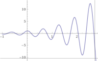
An example curve of et cos(10t) that is added together with similar curves to form a Laplace Transform.
Animation showing how adding together curves can approximate a function.
.png&filetimestamp=20221230192601&)

انظر أيضاً
الهامش
- ^ Lynn, Paul A. (1986). "The Laplace Transform and the z-transform". Electronic Signals and Systems. London: Macmillan Education UK. pp. 225–272. doi:10.1007/978-1-349-18461-3_6. ISBN 978-0-333-39164-8.
Laplace Transform and the z-transform are closely related to the Fourier Transform. Laplace Transform is somewhat more general in scope than the Fourier Transform, and is widely used by engineers for describing continuous circuits and systems, including automatic control systems.
- ^ "Differential Equations - Laplace Transforms". tutorial.math.lamar.edu. Retrieved 2020-08-08.
- ^ أ ب Weisstein, Eric W. "Laplace Transform". mathworld.wolfram.com (in الإنجليزية). Retrieved 2020-08-08.
- ^ "Des Fonctions génératrices" (in fr), Théorie analytique des Probabilités (2nd ed.), Paris, 1814, chap.I sect.2-20, https://archive.org/details/thorieanalytiqu01laplgoog
- ^ Jaynes, E. T. (Edwin T.) (2003). Probability theory : the logic of science. Bretthorst, G. Larry. Cambridge, UK: Cambridge University Press. ISBN 0511065892. OCLC 57254076.
- ^ Abel, Niels H. (1820), "Sur les fonctions génératrices et leurs déterminantes" (in fr), Œuvres Complètes, II (published 1839), pp. 77–88 1881 edition
- ^ Lerch, Mathias (1903), "Sur un point de la théorie des fonctions génératrices d'Abel" (in fr), Acta Mathematica 27: 339–351, doi:
- ^ Heaviside, Oliver (January 2008), "The solution of definite integrals by differential transformation", Electromagnetic Theory, III, London, section 526, ISBN 9781605206189
- ^ Bromwich, Thomas J. (1916), "Normal coordinates in dynamical systems", Proceedings of the London Mathematical Society 15: 401–448, doi:, https://zenodo.org/record/2319588
- ^ An influential book was: Gardner, Murray F.; Barnes, John L. (1942), Transients in Linear Systems studied by the Laplace Transform, New York: Wiley
- ^ Doetsch, Gustav (1937) (in de), Theorie und Anwendung der Laplacesche Transformation, Berlin: Springer translation 1943
- ^ Euler 1744, Euler 1753, Euler 1769
- ^ Lagrange 1773
- ^ Grattan-Guinness 1997, p. 260
- ^ Grattan-Guinness 1997, p. 261
- ^ Grattan-Guinness 1997, pp. 261–262
- ^ Grattan-Guinness 1997, pp. 262–266
- ^ Feller 1971, §XIII.1
- ^ Korn & Korn 1967, pp. 226–227
- ^ Bracewell 2000, Table 14.1, p. 385
- ^ Feller 1971, p. 432
- ^ Takacs 1953, p. 93
- ^ Riley, K. F.; Hobson, M. P.; Bence, S. J. (2010), Mathematical methods for physics and engineering (3rd ed.), Cambridge University Press, p. 455, ISBN 978-0-521-86153-3
- ^ Distefano, J. J.; Stubberud, A. R.; Williams, I. J. (1995), Feedback systems and control, Schaum's outlines (2nd ed.), McGraw-Hill, p. 78, ISBN 978-0-07-017052-0
- ^ Lipschutz, S.; Spiegel, M. R.; Liu, J. (2009). Mathematical Handbook of Formulas and Tables. Schaum's Outline Series (3rd ed.). McGraw-Hill. p. 183. ISBN 978-0-07-154855-7. – provides the case for real q.
- ^ http://mathworld.wolfram.com/LaplaceTransform.html – Wolfram Mathword provides case for complex q
- ^ أ ب ت ث Bracewell 1978, p. 227.
- ^ أ ب ت Williams 1973, p. 88.
- ^ أ ب Williams 1973, p. 89.
- ^ Korn & Korn 1967, §8.1
- ^ RK Pathria; Paul Beal (1996). Statistical mechanics (2nd ed.). Butterworth-Heinemann. p. 56. ISBN 9780750624695.
- ^ Salem, M.; Seaton, M. J. (1974), "I. Continuum spectra and brightness contours", Monthly Notices of the Royal Astronomical Society 167: 493–510, doi:, Bibcode: 1974MNRAS.167..493S, and
Salem, M. (1974), "II. Three-dimensional models", Monthly Notices of the Royal Astronomical Society 167: 511–516, doi:, Bibcode: 1974MNRAS.167..511S
المراجع
الحديثة
- Bracewell, Ronald N. (1978), The Fourier Transform and its Applications (2nd ed.), McGraw-Hill Kogakusha, ISBN 978-0-07-007013-4
- Bracewell, R. N. (2000), The Fourier Transform and Its Applications (3rd ed.), Boston: McGraw-Hill, ISBN 978-0-07-116043-8
- Feller, William (1971), An introduction to probability theory and its applications. Vol. II., Second edition, New York: John Wiley & Sons
- Korn, G. A.; Korn, T. M. (1967), Mathematical Handbook for Scientists and Engineers (2nd ed.), McGraw-Hill Companies, ISBN 978-0-07-035370-1
- Widder, David Vernon (1941), The Laplace Transform, Princeton Mathematical Series, v. 6, Princeton University Press
- Williams, J. (1973), Laplace Transforms, Problem Solvers, George Allen & Unwin, ISBN 978-0-04-512021-5
- Takacs, J. (1953), "Fourier amplitudok meghatarozasa operatorszamitassal" (in hu), Magyar Hiradastechnika IV (7–8): 93–96
التاريخية
- Euler, L. (1744), "De constructione aequationum" (in la), Opera Omnia, 1st series 22: 150–161
- Euler, L. (1753), "Methodus aequationes differentiales" (in la), Opera Omnia, 1st series 22: 181–213
- Euler, L. (1992), "Institutiones calculi integralis, Volume 2" (in la), Opera Omnia, 1st series (Basel: Birkhäuser) 12, ISBN 978-3764314743, Chapters 3–5
- Euler, Leonhard (1769) (in la), Institutiones calculi integralis, II, Paris: Petropoli, ch. 3–5, pp. 57–153, https://books.google.com/books?id=BFqWNwpfqo8C
- Grattan-Guinness, I (1997), "Laplace's integral solutions to partial differential equations", in Gillispie, C. C., Pierre Simon Laplace 1749–1827: A Life in Exact Science, Princeton: Princeton University Press, ISBN 978-0-691-01185-1
- Lagrange, J. L. (1773), Mémoire sur l'utilité de la méthode, Œuvres de Lagrange, 2, pp. 171–234
للاستزادة
- Arendt, Wolfgang; Batty, Charles J.K.; Hieber, Matthias; Neubrander, Frank (2002), Vector-Valued Laplace Transforms and Cauchy Problems, Birkhäuser Basel, ISBN 978-3-7643-6549-3.
- Davies, Brian (2002), Integral transforms and their applications (Third ed.), New York: Springer, ISBN 978-0-387-95314-4
- Deakin, M. A. B. (1981), "The development of the Laplace transform", Archive for History of Exact Sciences 25 (4): 343–390, doi:
- Deakin, M. A. B. (1982), "The development of the Laplace transform", Archive for History of Exact Sciences 26 (4): 351–381, doi:
- Doetsch, Gustav (1974), Introduction to the Theory and Application of the Laplace Transformation, Springer, ISBN 978-0-387-06407-9
- Mathews, Jon; Walker, Robert L. (1970), Mathematical methods of physics (2nd ed.), New York: W. A. Benjamin, ISBN 0-8053-7002-1
- Polyanin, A. D.; Manzhirov, A. V. (1998), Handbook of Integral Equations, Boca Raton: CRC Press, ISBN 978-0-8493-2876-3
- Schwartz, Laurent (1952), "Transformation de Laplace des distributions" (in fr), Comm. Sém. Math. Univ. Lund [Medd. Lunds Univ. Mat. Sem.] 1952: 196–206
- Schwartz, Laurent (2008), Mathematics for the Physical Sciences, Dover Books on Mathematics, New York: Dover Publications, pp. 215–241, ISBN 978-0-486-46662-0, https://books.google.com/books?id=-_AuDQAAQBAJ&pg=PA215 - See Chapter VI. The Laplace transform.
- Siebert, William McC. (1986), Circuits, Signals, and Systems, Cambridge, Massachusetts: MIT Press, ISBN 978-0-262-19229-3
- Widder, David Vernon (1945), "What is the Laplace transform?", The American Mathematical Monthly 52 (8): 419–425, doi:, ISSN 0002-9890
وصلات خارجية
- Hazewinkel, Michiel, ed. (2001), "Laplace transform", Encyclopaedia of Mathematics, Kluwer Academic Publishers, ISBN 978-1556080104
- Online Computation of the transform or inverse transform, wims.unice.fr
- Tables of Integral Transforms at EqWorld: The World of Mathematical Equations.
- Eric W. Weisstein, Laplace Transform at MathWorld.
- Good explanations of the initial and final value theorems Archived 2009-01-08 at the Wayback Machine
- Laplace Transforms at MathPages
- Computational Knowledge Engine allows to easily calculate Laplace Transforms and its inverse Transform.
- Laplace Calculator to calculate Laplace Transforms online easily.
- Code to visualize Laplace Transforms and many example videos.